library(tidyverse)
library(tidymodels)
library(gapminder)
From today’s class, students are anticipated to be able to:
- make a model object in R, using
lm()as an example. - write a formula in R.
- predict on a model object with the
broom::augment()andpredict()functions. - extract information from a model object using
broom::tidy(),broom::glance(), and traditional means.
Note that there is a new tidyverse-like framework of packages to help with modelling. It’s called tidymodels.
Resources
Video lecture:
Other resources, in addition to the notes below:
- The broom vignette is useful for learning the details of broom, a package for tidying the output of models.
- If you want a quick intro to linear regression with R, check out this U Chicago Tutorial on model fitting in R (just the linear regression part).
- If you’re eager to learn more about models in general, An Introduction to Statistical Learning is an approachable read (the book is freely available online)
- Mike Marin’s R playlist on YouTube helps you use R to obtain statistical results.
Model-fitting in R
Data wrangling and plotting can get you pretty far when it comes to drawing insight from your data. But, sometimes you need to go further. For example:
- Investigate the relationship between two or more variables
- Predict the outcome of a variable given information about other variables
These typically involve fitting models, as opposed to simple computations than can be done with tidyverse packages like dplyr.
This tutorial is not about the specifics of fitting a model. Even though a few references to statistical concepts are made, just take these for face value.
Example: linear model
Here are a couple tasks that model-fitting would be useful to address.
- A car weighs 4000 lbs. Provide a numerical prediction on its mpg (miles per gallon).
- Does the weight of a car influence its mpg?
- How many more miles per gallon can we expect of a car that weighs 1000 lbs less than another car?
A simple scatterplot will give us a general idea, but can’t give us specifics. Here, we use the mtcars dataset in the datasets package. A linear model is one example of a model that can attempt to answer all three – the line corresponding to the fitted model has been added to the scatterplot.
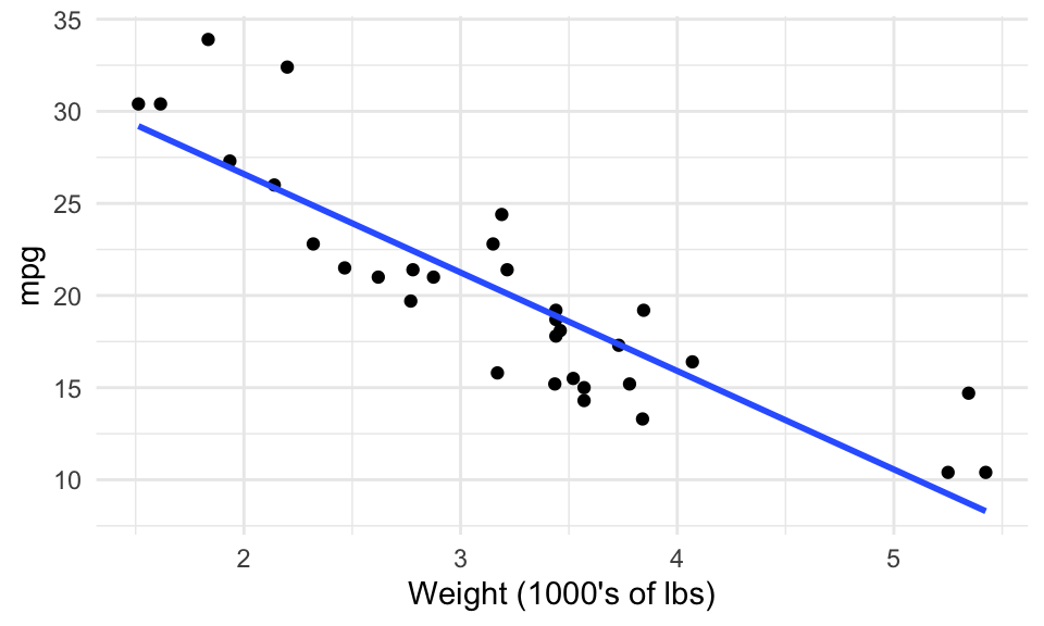
(By the way, you can plot the model using ggplot2’s geom_smooth() layer – but you can’t interact with the model downstream.)
We can make a prediction of mpg for a car weighing 3,000 lbs by evaluating the line at X = 3:
## [1] 21.25171We can find the p-value testing the null hypothesis that the true slope of the regression line is 0:
## [1] 1.293959e-10And we can calculate how many more miles per gallon a car weighing 1000 less lbs would be expected to have through the slope:
## [1] 5.344472Fitting a model in R
Fitting a model in R typically involves using a function in the following format:
method(formula, data, options)Method:
A function such as:
- Linear Regression:
lm - Generalized Linear Regression:
glm - Local regression:
loess - Quantile regression:
quantreg::rq - …
Formula:
In R, takes the form y ~ x1 + x2 + ... + xp (use column names in your data frame), where y here means the outcome variable you’re interested in viewing in relation to other variables x1, x2, …
Data: The data frame or tibble. Can omit, if variables in the formula are defined in environment
Options: Specific to the method, and include ways to customize the model.
Running the code returns an object – usually a special type of list – that you can then work with to extract results.
For example, let’s fit a linear regression model on a car’s mileage per gallon (mpg, “Y” variable) from the car’s weight (wt, “X” variable). Notice that no special options are needed for lm().
(my_lm <- lm(mpg ~ wt, data = mtcars))##
## Call:
## lm(formula = mpg ~ wt, data = mtcars)
##
## Coefficients:
## (Intercept) wt
## 37.285 -5.344Printing the model to the screen might lead you to incorrectly conclude that the model object my_lm only contains the above text. The reality is, my_lm contains a lot more, but special instructions have been given to R to only print out a special digested version of the object. This behaviour tends to be true with model objects in general, not just for lm().
Probing the model: Broom
Now that you have the model object, there are typically three ways in which it’s useful to probe and use the model object. The broom package has three crown functions that make it easy to extract each piece of information by converting your model into a tibble:
tidy: extract statistical summaries about each “component” of the model.augment: add columns to the original data frame containing predictions.glance: extract statistical summaries about the model as a whole (a 1-row tibble).
tidy()
Use the tidy() function for a statistical summary of each component of your model, where each component gets a row in the output tibble. For lm(), tidy() gives one row per regression coefficient (slope and intercept).
tidy(my_lm)## # A tibble: 2 × 5
## term estimate std.error statistic p.value
## <chr> <dbl> <dbl> <dbl> <dbl>
## 1 (Intercept) 37.3 1.88 19.9 8.24e-19
## 2 wt -5.34 0.559 -9.56 1.29e-10tidy() only works if it makes sense to talk about model “components”.
augment()
Use the augment() function to make predictions on a dataset by augmenting predictions as a new column to your data. By default, augment() uses the dataset that was used to fit the model.
augment(my_lm) %>%
  print(n = 5)
## # A tibble: 32 × 9
## .rownames mpg wt .fitted .resid .hat .sigma .cooksd .std.resid
## <chr> <dbl> <dbl> <dbl> <dbl> <dbl> <dbl> <dbl> <dbl>
## 1 Mazda RX4 21 2.62 23.3 -2.28 0.0433 3.07 1.33e-2 -0.766
## 2 Mazda RX4 Wag 21 2.88 21.9 -0.920 0.0352 3.09 1.72e-3 -0.307
## 3 Datsun 710 22.8 2.32 24.9 -2.09 0.0584 3.07 1.54e-2 -0.706
## 4 Hornet 4 Drive 21.4 3.22 20.1 1.30 0.0313 3.09 3.02e-3 0.433
## 5 Hornet Sportabout 18.7 3.44 18.9 -0.200 0.0329 3.10 7.60e-5 -0.0668
## # ℹ 27 more rowsWe can also predict on new datasets. Here are predictions of mpg for cars weighing 3, 4, and 5 thousand lbs.
augment(my_lm, newdata = tibble(wt = 3:5))## # A tibble: 3 × 2
## wt .fitted
## <int> <dbl>
## 1 3 21.3
## 2 4 15.9
## 3 5 10.6Notice that only the “X” variables are needed in the input tibble (wt), and that since the “Y” variable (mpg) wasn’t provided, augment() couldn’t calculate anything besides a prediction.
glance()
Use the glance() function to extract a summary of the model as a whole, in the form of a one-row tibble. This will give you information related to the model fit.
glance(my_lm)## # A tibble: 1 × 12
## r.squared adj.r.squared sigma statistic p.value df logLik AIC BIC
## <dbl> <dbl> <dbl> <dbl> <dbl> <dbl> <dbl> <dbl> <dbl>
## 1 0.753 0.745 3.05 91.4 1.29e-10 1 -80.0 166. 170.
## # ℹ 3 more variables: deviance <dbl>, df.residual <int>, nobs <int>Probing the Model: Traditional Method
In order for a model to work with the broom package, someone has to go out of their way to contribute to the broom package for that model. While this has happened for many common models, many others remain without broom compatibility.
Here’s how to work with these model objects in that case.
Prediction
If broom::augment() doesn’t work, then the developer of the model almost surely made it so that the predict() function works (not part of the broom package). The predict() function typically takes the same format of the augment() function, but usually doesn’t return a tibble.
Here are the first 5 predictions of mpg on the my_lm object, defaulting to predictions made on the original data:
predict(my_lm) %>%
  unname() %>%
  head(5)
## [1] 23.28261 21.91977 24.88595 20.10265 18.90014Here are the predictions of mpg made for cars with a weight of 3, 4, and 5 thousand lbs:
predict(my_lm, newdata = tibble(wt = 3:5)) %>%
  unname()
## [1] 21.25171 15.90724 10.56277Checking the documentation of the predict() function for your model isn’t obvious, because the predict() function is a “generic” function. Your best bet is to append the model name after a dot. For example:
- For a model fit with
lm(), try?predict.lm - For a model fit with
rq(), try?predict.rq(from thequantregpackage)
If that doesn’t work, just google it: "Predict function for rq"
Functions designed for the model
The developer of the model probably made a suite of other functions to help you probe the model object. Check the documentation to find these.
For example, I can find the regression coefficients of a lm() object with coef():
coef(my_lm)## (Intercept) wt
## 37.285126 -5.344472Standard error of the residuals with sigma():
sigma(my_lm)## [1] 3.045882Don’t be surprised if there is no function to extract what you want. If that’s the case, read on…
Manually Extracting Information
If you can’t extract model information from built-in functions like coef() or sigma(), you can manually dig in to the model object. In most cases, a model object is just a list in disguise! (Lists are discussed in STAT 545B). You can therefore extract information like you would with any other list.
To help figure out what’s in the list, use the names() function. Here are all the entries in the lm() object we fit earlier:
names(my_lm)## [1] "coefficients" "residuals" "effects" "rank"
## [5] "fitted.values" "assign" "qr" "df.residual"
## [9] "xlevels" "call" "terms" "model"Want the degrees of freedom of the residuals? Just extract that entry:
my_lm$df.residual## [1] 30To complicate things further this might only be part of the information made available in the model object! More info might be stored in yet another list after applying the summary() function:
summary(my_lm)##
## Call:
## lm(formula = mpg ~ wt, data = mtcars)
##
## Residuals:
## Min 1Q Median 3Q Max
## -4.5432 -2.3647 -0.1252 1.4096 6.8727
##
## Coefficients:
## Estimate Std. Error t value Pr(>|t|)
## (Intercept) 37.2851 1.8776 19.858 < 2e-16 ***
## wt -5.3445 0.5591 -9.559 1.29e-10 ***
## ---
## Signif. codes: 0 '***' 0.001 '**' 0.01 '*' 0.05 '.' 0.1 ' ' 1
##
## Residual standard error: 3.046 on 30 degrees of freedom
## Multiple R-squared: 0.7528, Adjusted R-squared: 0.7446
## F-statistic: 91.38 on 1 and 30 DF, p-value: 1.294e-10Like the original model object, summary() looks like it returns a bunch of text – but it’s actually another list! Let’s again use names() to get the components of this list:
names(summary(my_lm))## [1] "call" "terms" "residuals" "coefficients"
## [5] "aliased" "sigma" "df" "r.squared"
## [9] "adj.r.squared" "fstatistic" "cov.unscaled"Now I can get more pieces of information, like the adjusted R-squared value:
summary(my_lm)$adj.r.squared## [1] 0.7445939Plotting models with geom_smooth
We can plot models (with one predictor/ X variable) using ggplot2 through the geom_smooth() layer. Specifying method="lm" gives us the linear regression fit (but only visually – very difficult to extract model components!):
ggplot(mtcars, aes(x = wt, y = mpg)) +
    geom_point() +
geom_smooth(method = "lm") ## `geom_smooth()` using formula = 'y ~ x'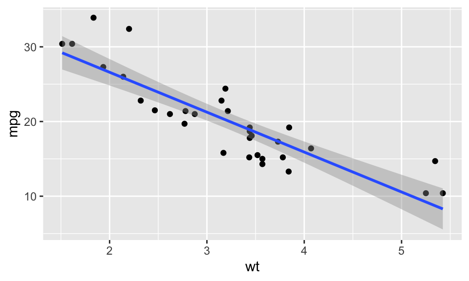
Let’s visualize some relationships in the gapminder dataset.
Let’s inspect Zimbabwe, which has a unique behavior in the lifeExp and year relationship.
gapminder_Zimbabwe <- gapminder %>%
filter(country == "Zimbabwe")
gapminder_Zimbabwe %>%
ggplot(aes(year, lifeExp)) +
geom_point()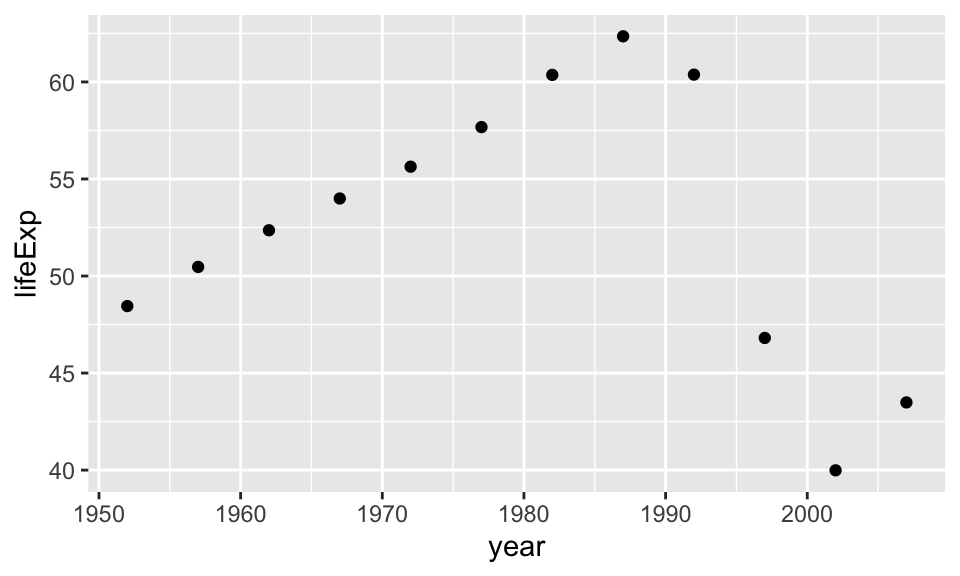 Let’s try fitting a linear model to this relationship
ggplot(gapminder_Zimbabwe, aes(year,lifeExp)) +
  geom_point() +
geom_smooth(method = "lm", se = F)## `geom_smooth()` using formula = 'y ~ x'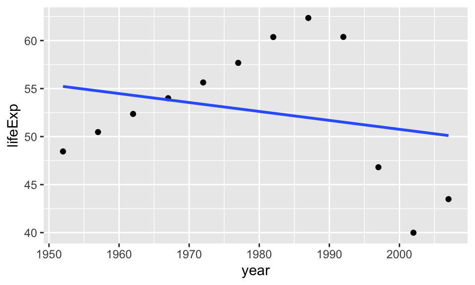 Now we will try to fit a second degree polynomial and see what would that look like.
ggplot(gapminder_Zimbabwe, aes(year,lifeExp)) +
  geom_point() +
  geom_smooth(method = "lm",
              formula = y ~ poly(x,2),
              se = F)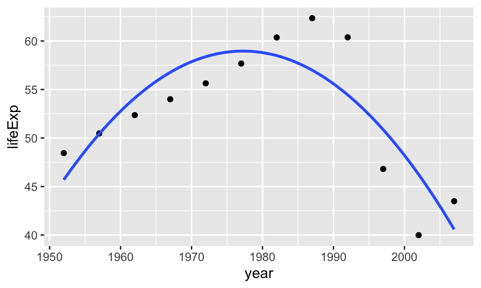
Summary
function(formula, data, options)- most models in R follow this structure.broom::augment()- uses a fitted model to obtain predictions. Puts this in a new column in existingtibble. Equivalent base-r function ispredict().broom::tidy()- used to extract statistical information on each component of a model. Equivalent iscoef(summary(lm_object)).broom::glance()- used to extract statistical summaries on the whole model. Always returns a 1-rowtibble.geom_smooth()- used to add geom_layer that shows a fitted line to the data.methodandformulaarguments can be used to customize model.
Test Your Understanding
- TRUE or FALSE: the output of
glanceon the above returns only 1 row because there is only 1 explanatory variable in the model. - TRUE or FALSE: the output of
broom::tidy()package is more “tidy” thancoef(summary())because the output is atibble - TRUE or FALSE: We need to use a modelling function, such as
lm, before we can graph a fitted line withgeom_smooth. - TRUE or FALSE: If I wanted to find the amount that
lifeExpchanges peryear, then I need to usebroom::tidy()
Your turn: learning to fit models in R
We think the best way to learn the basics from here is to work through the last part of Worksheet A4.
In-class Schedule
First part
- Attempt questions on the last part of Worksheet A4
- Get answers about questions you got stuck on
Second part
While this is not a modelling class, let’s get a sense of where modelling would fit into a real data analysis by working through the final part of the FEV case study.
Attribution
Model fitting intro by Vincenzo Coia with input from Victor Yuan. FEV case study added later by Lucy.