Review
We’ll continue exploring the FEV data set. Let’s start by loading the data and required packages.
library(rigr)
library(tidyverse)
library(broom)

fev_tbl <- as_tibble(fev) %>% mutate(across(sex:smoke, ~ as.factor(.x)))
Previously, we found that the mean FEV in the smoking group was substantially higher than the average FEV in the non-smoking group; this speaks to the unadjusted association between smoking and lung function. But we also found that the FEV of smokers and non-smokers of the same height is pretty similar; that is, there doesn’t seem to be much of an association between smoking and lung function, when adjusted for height. We also found other factors in the data set seemingly related to smoking status, FEV, or both that we might like to adjust for, like age and sex.
A simple two group model
We previously calculated the mean FEV among the smokers and the non-smokers in our data set.
fev_tbl %>% group_by(smoke) %>%
  summarize(mean_fev = mean(fev), sd_fev = sd(fev), n = n())
## # A tibble: 2 × 4
## smoke mean_fev sd_fev n
## <fct> <dbl> <dbl> <int>
## 1 no 2.57 0.851 589
## 2 yes 3.28 0.750 65These are estimates of the mean FEV among the whole population of smokers and the population of non-smokers, calculated using our data. Are the population mean FEVs different? How different? We can get an answer to these questions by not just estimating population mean FEVs, but also performing statistical inference on the difference between the population mean FEVs. To do this, we’ll use the t.test() function built into R to perform a two-sample t-test.
(tt_fev <- t.test(fev ~ smoke, fev_tbl, var.equal=FALSE))##
## Welch Two Sample t-test
##
## data: fev by smoke
## t = -7.1496, df = 83.273, p-value = 3.074e-10
## alternative hypothesis: true difference in means between group no and group yes is not equal to 0
## 95 percent confidence interval:
## -0.9084253 -0.5130126
## sample estimates:
## mean in group no mean in group yes
## 2.566143 3.276862If I felt like being extremely careful, then here is how I would describe the results of this test.
“In the FEV data set, the mean FEV among children who do not smoke was 2.6 L/s and the mean FEV among children who smoke was 3.3 L/s in children. The data are consistent with the population mean FEV among children who smoke being between 0.5 L/s and 0.9 L/s higher than the population mean FEV among children who do not smoke. We reject the null hypothesis of no difference in the population mean FEV among children who smoke and children who do not smoke (p < 0.0001).”
In practice, what you will see in scientific reports will typically be much more brief.
Exercise 1
Use the tidy() function to extract the information printed above into a tibble. Then, practice manually extracting the p-value and lower and upper confidence limits.
tidy(tt_fev)## # A tibble: 1 × 10
## estimate estimate1 estimate2 statistic p.value parameter conf.low conf.high
## <dbl> <dbl> <dbl> <dbl> <dbl> <dbl> <dbl> <dbl>
## 1 -0.711 2.57 3.28 -7.15 3.07e-10 83.3 -0.908 -0.513
## # ℹ 2 more variables: method <chr>, alternative <chr>tt_fev$p.value## [1] 3.073813e-10tt_fev$conf.int## [1] -0.9084253 -0.5130126
## attr(,"conf.level")
## [1] 0.95Fitting a simple linear model
We previously made this scatterplot of FEV versus height, with points coloured by smoking status. Based on this plot, it seems like the FEV of smokers and non-smokers of the same height is pretty similar.
(scatter_fev <- ggplot(fev_tbl, aes(x = height, y = fev, colour=smoke)) +
  geom_jitter(width=0.2, alpha = 0.75) +
  scale_colour_manual(values=c("cornflowerblue","darkorange")) +
  ggtitle("FEV versus height, stratified by smoking status") +
  ylab("FEV (l/s)") +
  xlab("Height (inches)") +
  theme_bw())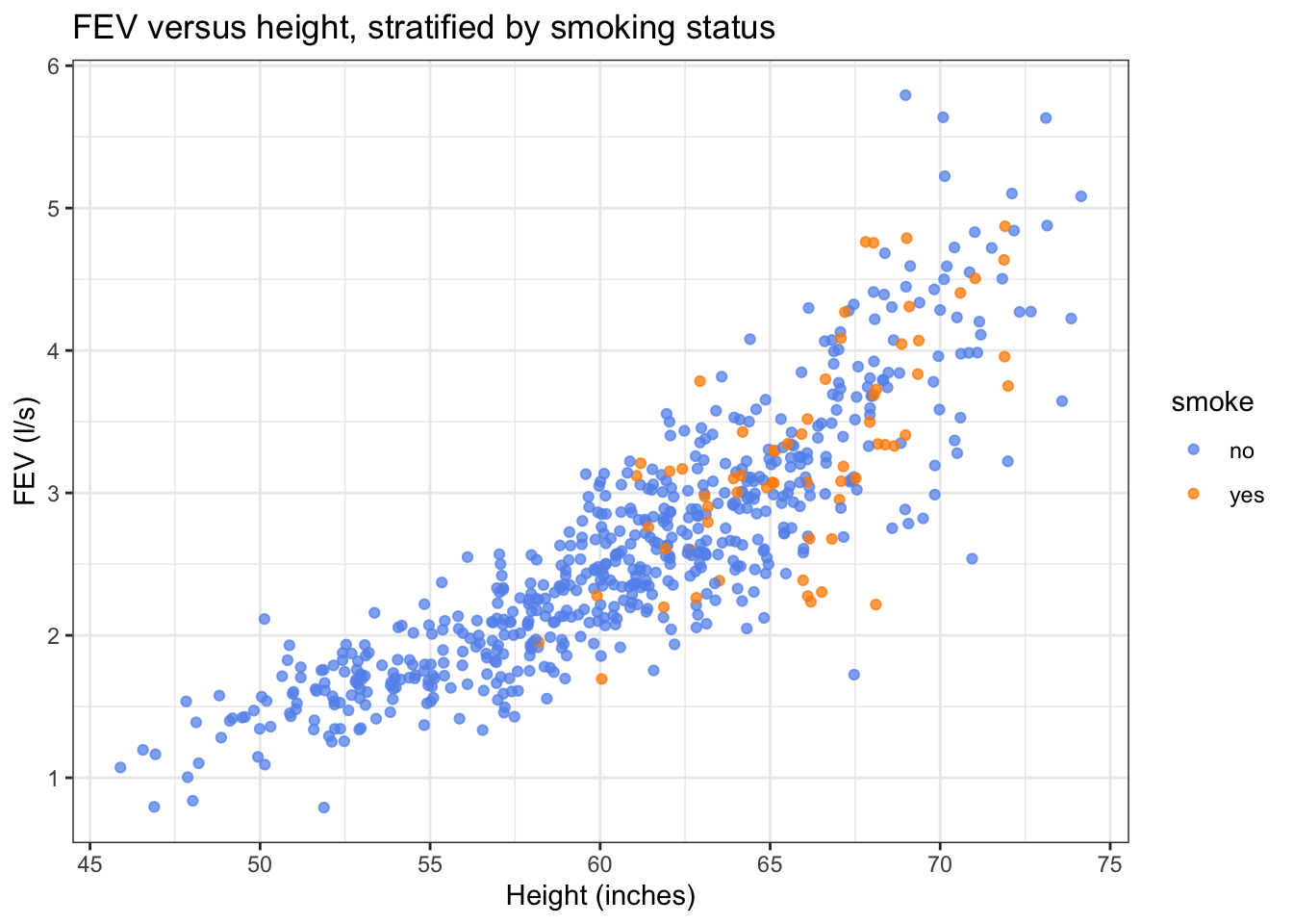
Exercise 2
Let’s fit simple linear models to the smokers and the non-smokers and add it to your plot. Hint: geom_smooth().
scatter_fev + geom_smooth(method="lm")## `geom_smooth()` using formula = 'y ~ x'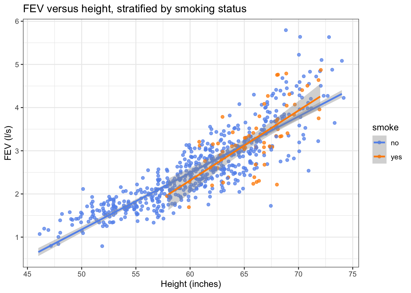
Notice how this makes it easier for us to compare the estimated mean FEV at different heights in the two groups.
Fitting a linear model with more variables
Exercise 3
Fit a linear model on the FEV from the smoking status, age, height, and sex.
(fev_lm <- lm(fev~smoke+age+height+sex, data=fev_tbl))##
## Call:
## lm(formula = fev ~ smoke + age + height + sex, data = fev_tbl)
##
## Coefficients:
## (Intercept) smokeyes age height sexmale
## -4.45697 -0.08725 0.06551 0.10420 0.15710Then, use the tidy() function to extract the information printed above (plus more!) into a tibble.
tidy(fev_lm)## # A tibble: 5 × 5
## term estimate std.error statistic p.value
## <chr> <dbl> <dbl> <dbl> <dbl>
## 1 (Intercept) -4.46 0.223 -20.0 1.07e-69
## 2 smokeyes -0.0872 0.0593 -1.47 1.41e- 1
## 3 age 0.0655 0.00949 6.90 1.21e-11
## 4 height 0.104 0.00476 21.9 4.98e-80
## 5 sexmale 0.157 0.0332 4.73 2.74e- 6