Learning Objectives
From today’s class, students are anticipated to be able to:
- Recognize how to manipulate data through a variety of tibble joins such as:
- Mutating joins:
left_join(),right_join(),full_join(),anti_join() - Filtering joins:
semi_join(),anti_join()
- Mutating joins:
- Perform binding:
bind_rows(),bind_cols() - Join more than 2 tibbles
- Join based on multiple conditions
- Perform set operations on data:
intersect(),union(),setdiff() - Join tibbles with different types of variables
Resources
Video lecture:
Demonstration .Rmd file:
Other resources, in addition to the notes below:
- Two-table verbs vignette
- Jenny’s Join Cheatsheet for a quick reference to joins.
- Relational Data chapter in “R for Data Science”.
- dplyr cheatsheet
Overview of join functions
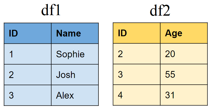
Note: In order to merge two tibbles, you need to have an identifier variable that has unique values for every row of observations in both tibbles.
Create two sample tibbles:
# First tibble
df1 <- tibble(ID = 1:3,
              Name = c("Sophie", "Josh","Alex"))

# Second tibble
df2 <- tibble(ID = 2:4,
              Age = c(20,50,31))
Mutating joins
Join matching rows from df2 to df1
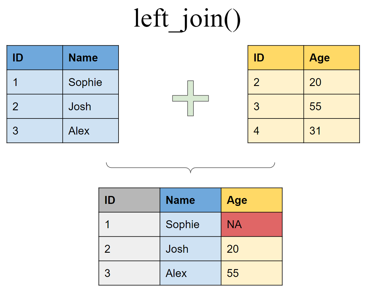
left_join(df1, df2, by = "ID")
## # A tibble: 3 x 3
##      ID Name     Age
##   <int> <chr>  <dbl>
## 1     1 Sophie    NA
## 2     2 Josh      20
## 3     3 Alex      50
Join matching rows from df1 to df2
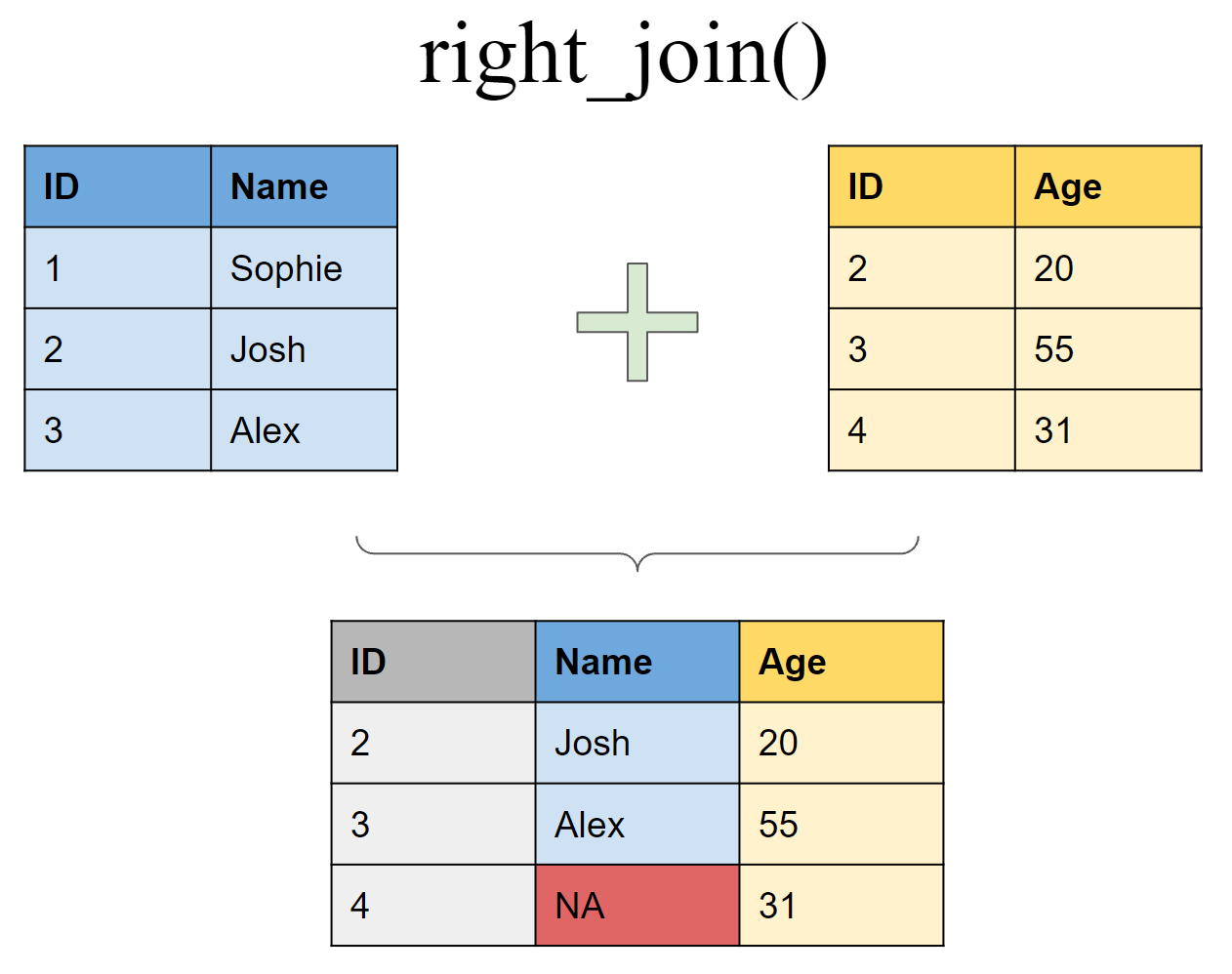
right_join(df1, df2, by = "ID")
## # A tibble: 3 x 3
##      ID Name    Age
##   <int> <chr> <dbl>
## 1     2 Josh     20
## 2     3 Alex     50
## 3     4 <NA>     31
Retain only rows present in both sets
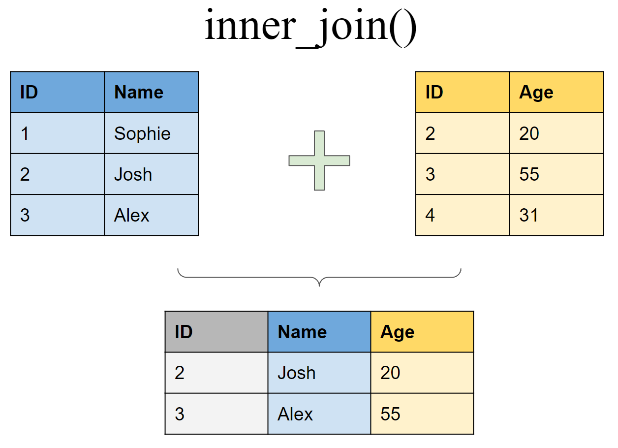
inner_join(df1, df2, by = "ID")
## # A tibble: 2 x 3
##      ID Name    Age
##   <int> <chr> <dbl>
## 1     2 Josh     20
## 2     3 Alex     50
Retain all values, all rows
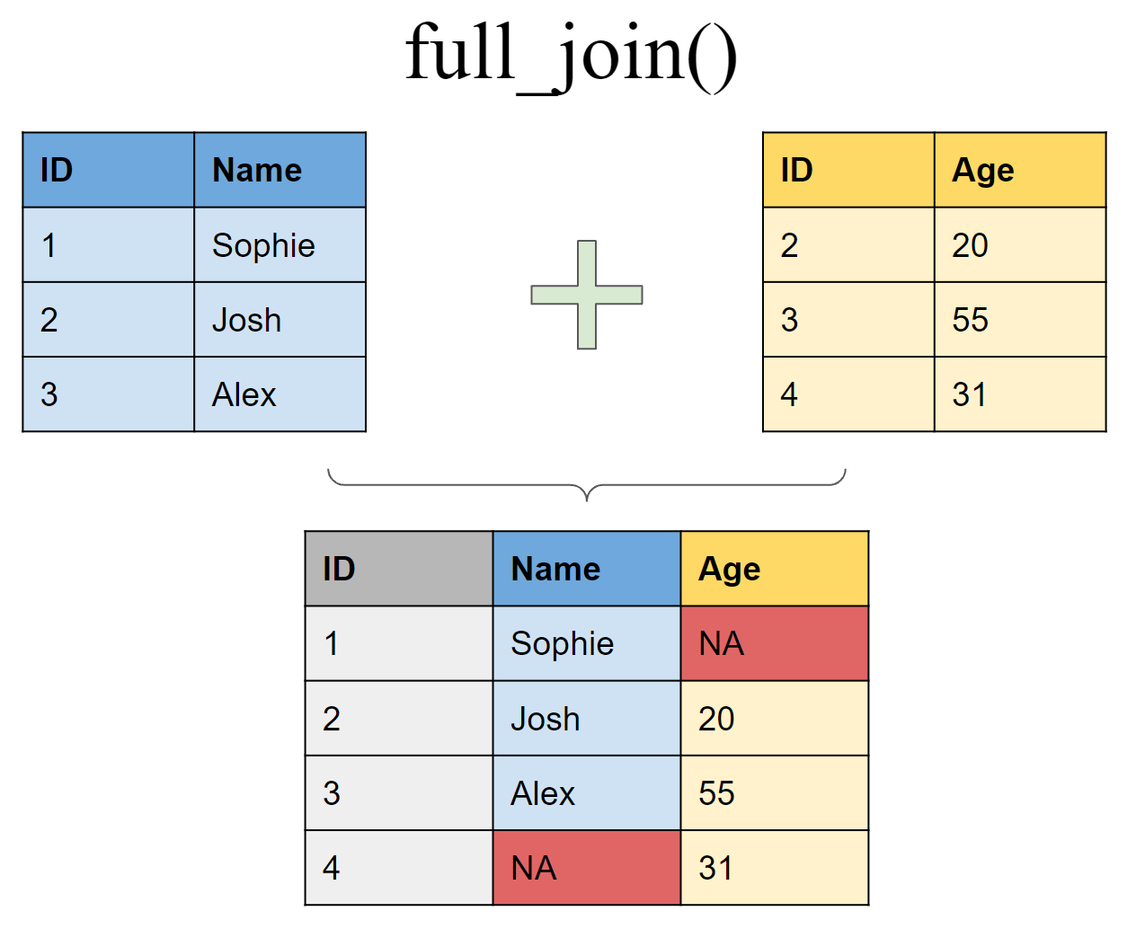
full_join(df1, df2, by = "ID")
## # A tibble: 4 x 3
##      ID Name     Age
##   <int> <chr>  <dbl>
## 1     1 Sophie    NA
## 2     2 Josh      20
## 3     3 Alex      50
## 4     4 <NA>      31
Filtering joins
Retain all rows in df1 that have a match in df2
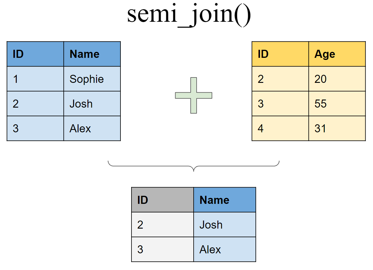
semi_join(df1, df2, by = "ID")
## # A tibble: 2 x 2
##      ID Name
##   <int> <chr>
## 1     2 Josh
## 2     3 Alex
Retain all rows in df1 that do not have a match in df2
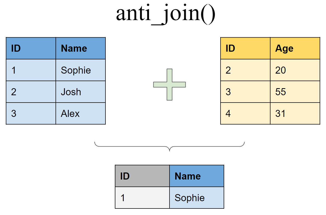
anti_join(df1, df2, by = "ID")
## # A tibble: 1 x 2
##      ID Name
##   <int> <chr>
## 1     1 Sophie
Binding
Append df2 to df1 as new rows
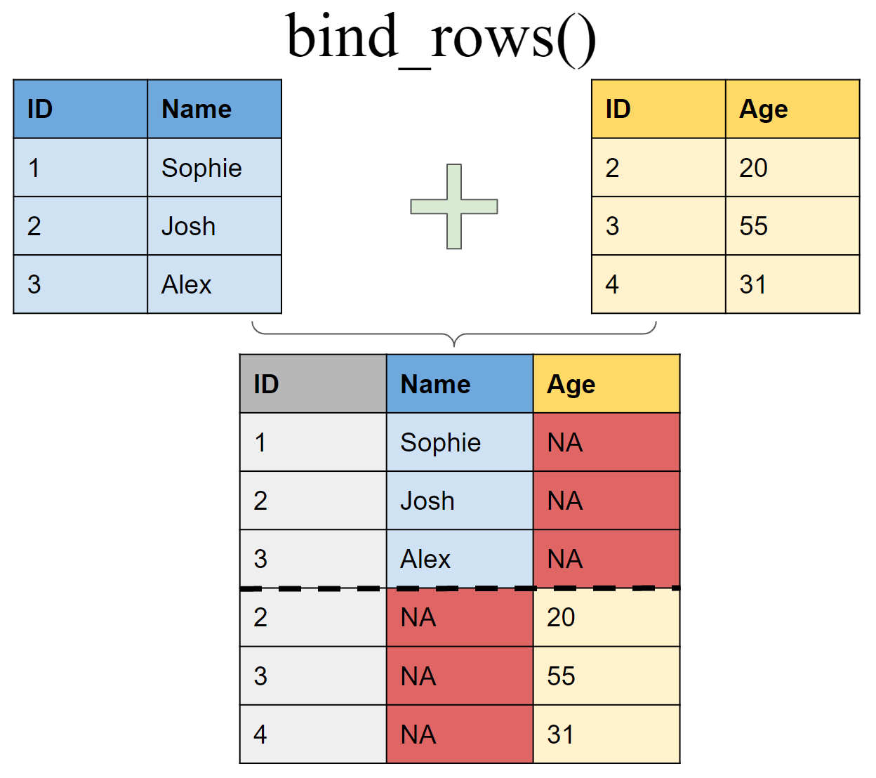
bind_rows(df1, df2)
## # A tibble: 6 x 3
##      ID Name     Age
##   <int> <chr>  <dbl>
## 1     1 Sophie    NA
## 2     2 Josh      NA
## 3     3 Alex      NA
## 4     2 <NA>      20
## 5     3 <NA>      50
## 6     4 <NA>      31
Append df2 to df1 as new columns
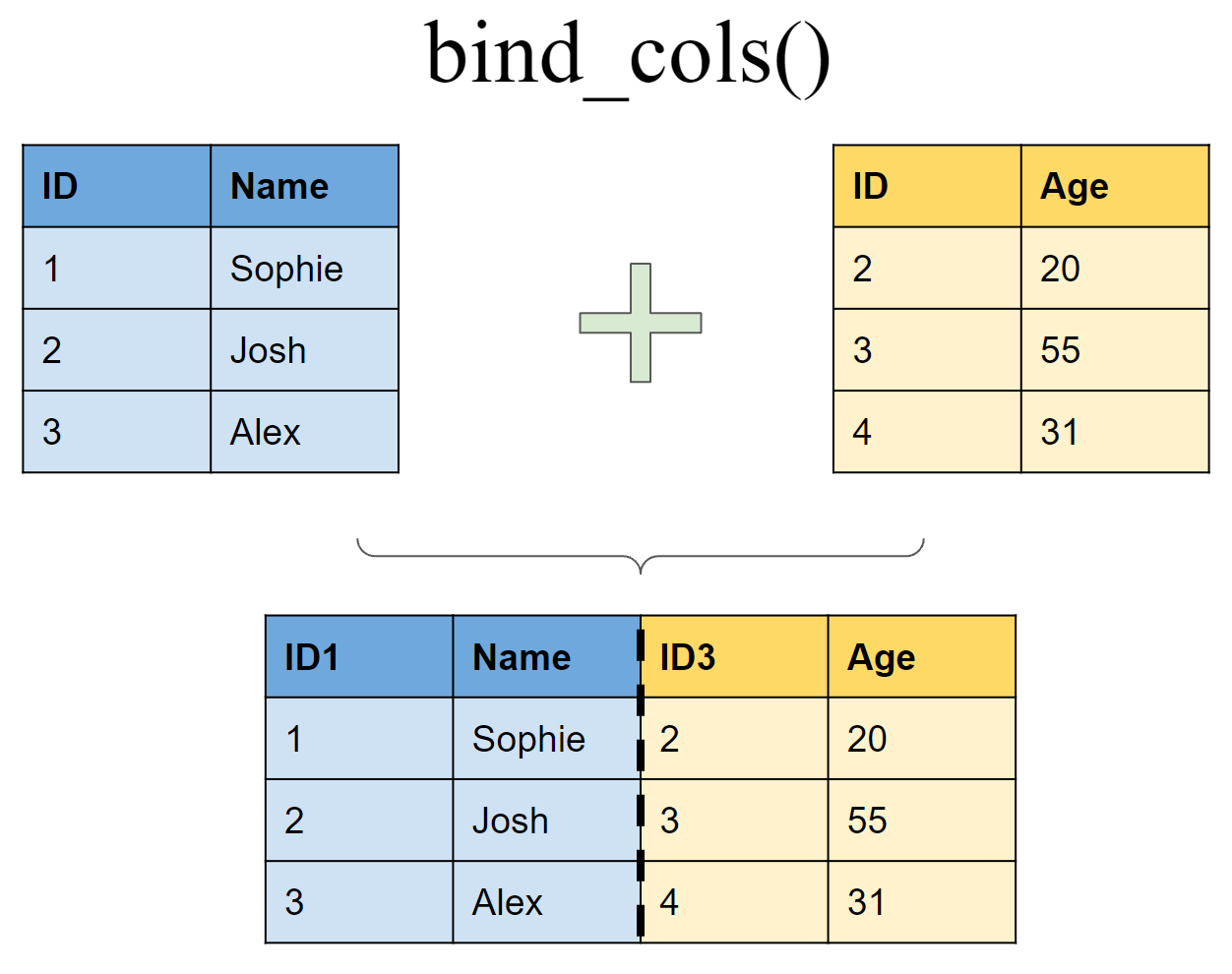
bind_cols(df1, df2)
## New names:
## * ID -> ID...1
## * ID -> ID...3

## # A tibble: 3 x 4
##   ID...1 Name   ID...3   Age
##    <int> <chr>   <int> <dbl>
## 1      1 Sophie      2    20
## 2      2 Josh        3    50
## 3      3 Alex        4    31
Joining multiple (>2) tibbles
Create a third tibble
df3 <- tibble(ID = 1:5,
              Height = c(175,167,190,155,160))
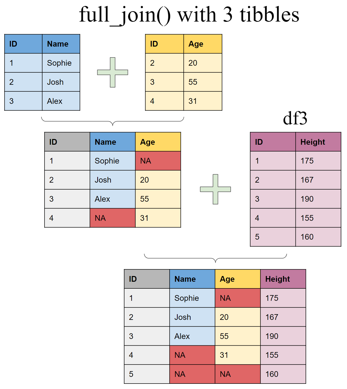
Use piping operator (%>%) to layer multiple join functions
full_join(df1, df2, by = "ID") %>%
  full_join(df3, by = "ID")
## # A tibble: 5 x 4
##      ID Name     Age Height
##   <int> <chr>  <dbl>  <dbl>
## 1     1 Sophie    NA    175
## 2     2 Josh      20    167
## 3     3 Alex      50    190
## 4     4 <NA>      31    155
## 5     5 <NA>      NA    160
Joining tibbles on multiple conditions
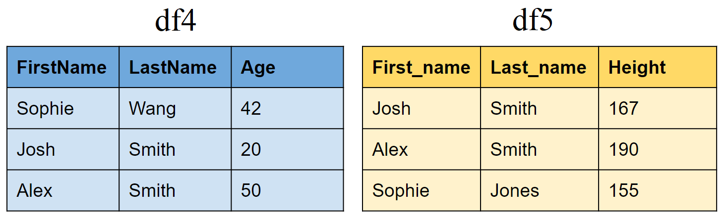
Create two new tibbles df4 and df5
df4 <- tibble(FirstName = c("Sophie", "Josh","Alex"),
              LastName=c("Wang","Smith","Smith"),
              Age = c(42,20,50))

df5 <- tibble(First_name = c("Josh","Alex","Sophie"),
              Last_name=c("Smith","Smith","Jones"),
              Height = c(167,190,155))
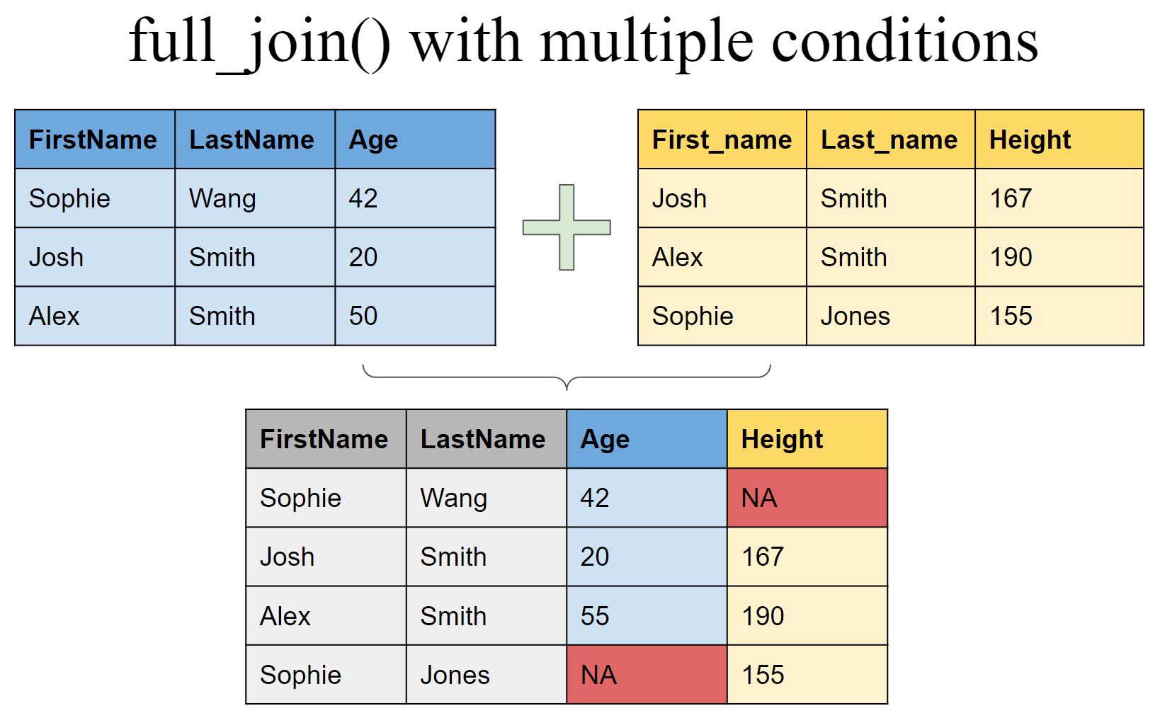
full_join(df4, df5, by = c("FirstName" = "First_name", "LastName" = "Last_name"))
## # A tibble: 4 x 4
##   FirstName LastName   Age Height
##   <chr>     <chr>    <dbl>  <dbl>
## 1 Sophie    Wang        42     NA
## 2 Josh      Smith       20    167
## 3 Alex      Smith       50    190
## 4 Sophie    Jones       NA    155
What if you did not realize that multiple people shared the same Last Name?
full_join(df4, df5, by = c("LastName" = "Last_name"))
## # A tibble: 6 x 5
##   FirstName LastName   Age First_name Height
##   <chr>     <chr>    <dbl> <chr>       <dbl>
## 1 Sophie    Wang        42 <NA>           NA
## 2 Josh      Smith       20 Josh          167
## 3 Josh      Smith       20 Alex          190
## 4 Alex      Smith       50 Josh          167
## 5 Alex      Smith       50 Alex          190
## 6 <NA>      Jones       NA Sophie        155
What if you did not realize that multiple people shared the same First Name?
full_join(df4, df5, by = c("FirstName" = "First_name"))
## # A tibble: 3 x 5
##   FirstName LastName   Age Last_name Height
##   <chr>     <chr>    <dbl> <chr>      <dbl>
## 1 Sophie    Wang        42 Jones        155
## 2 Josh      Smith       20 Smith        167
## 3 Alex      Smith       50 Smith        190
Set operations
Create sample tibbles
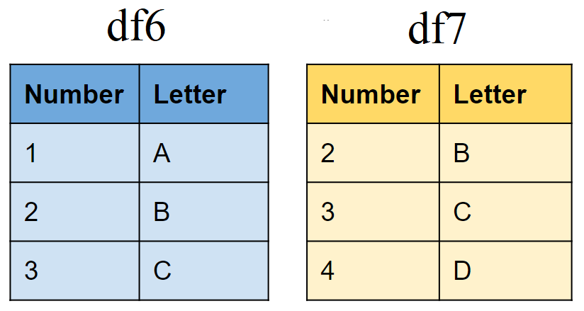
# First tibble
df6 <- tibble(Number = 1:3,
              Letter = c("A", "B","C"))

# Second tibble
df7 <- tibble(Number = 2:4,
              Letter = c("B","C","D"))
Include rows that appear in both tibbles
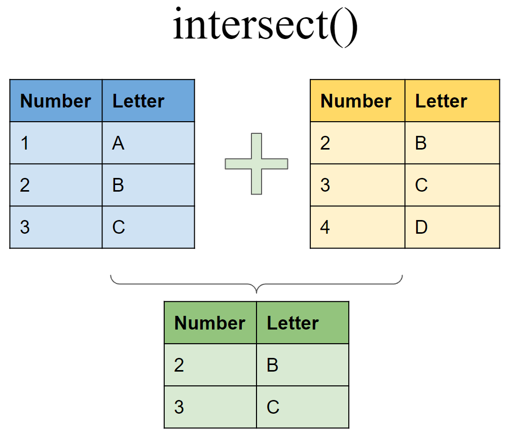
intersect(df6, df7)
## # A tibble: 2 x 2
##   Number Letter
##    <int> <chr>
## 1      2 B
## 2      3 C
Include rows that appear in either or both tibbles
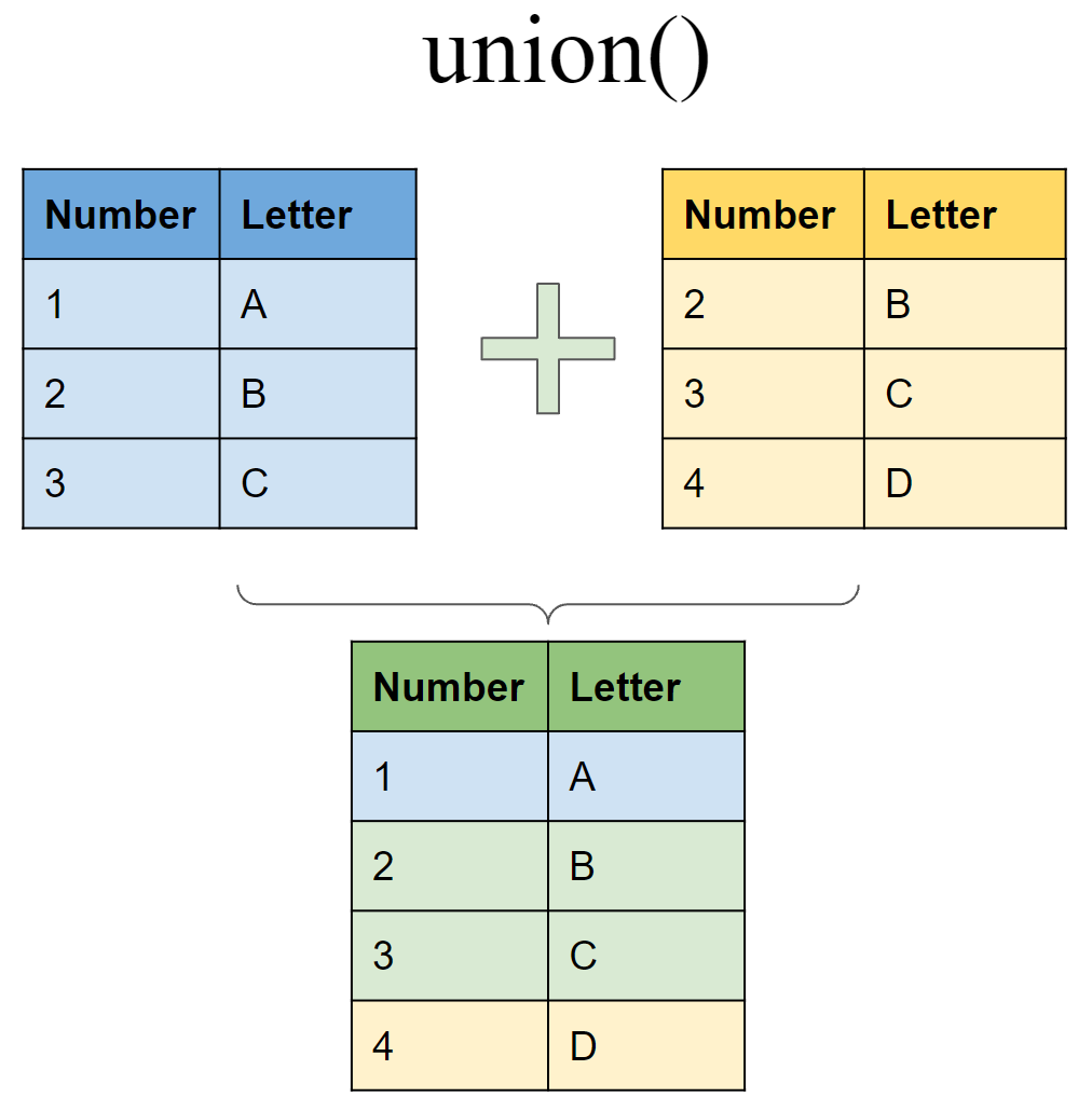
union(df6, df7)
## # A tibble: 4 x 2
##   Number Letter
##    <int> <chr>
## 1      1 A
## 2      2 B
## 3      3 C
## 4      4 D
Include rows that appear in one df but not another
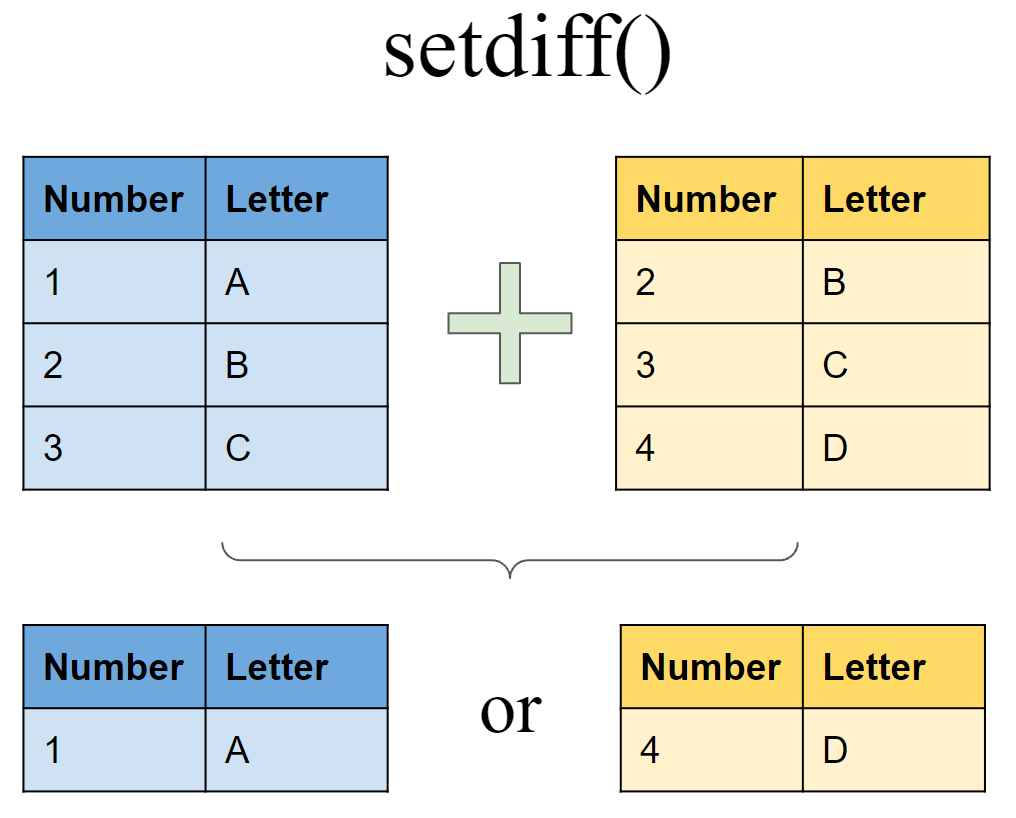
Include rows that appear in df6 but not in df7
setdiff(df6, df7)
## # A tibble: 1 x 2
##   Number Letter
##    <int> <chr>
## 1      1 A
Include rows that appear in df7 but not in df6
setdiff(df7, df6)
## # A tibble: 1 x 2
##   Number Letter
##    <int> <chr>
## 1      4 D
Joining tibbles with different types of variables
You can also join tibbles with sets of predictions:
set.seed(1)
x <- rnorm(5)
model1 <- tibble(x = x, yhat = 2.1 + 3.2 * x)
model2 <- tibble(x = x, yhat = 1.5 + 2.9 * x)
left_join(model1, model2, by = "x")
## # A tibble: 5 x 3
##        x  yhat.x yhat.y
##    <dbl>   <dbl>  <dbl>
## 1 -0.626  0.0953 -0.317
## 2  0.184  2.69    2.03
## 3 -0.836 -0.574  -0.923
## 4  1.60   7.20    6.13
## 5  0.330  3.15    2.46
Demonstration with gapminder
Get an overview of gapminder data
glimpse(gapminder)
## Rows: 1,704
## Columns: 6
## $ country   <fct> "Afghanistan", "Afghanistan", "Afghanistan", "Afghanistan", ~
## $ continent <fct> Asia, Asia, Asia, Asia, Asia, Asia, Asia, Asia, Asia, Asia, ~
## $ year      <int> 1952, 1957, 1962, 1967, 1972, 1977, 1982, 1987, 1992, 1997, ~
## $ lifeExp   <dbl> 28.801, 30.332, 31.997, 34.020, 36.088, 38.438, 39.854, 40.8~
## $ pop       <int> 8425333, 9240934, 10267083, 11537966, 13079460, 14880372, 12~
## $ gdpPercap <dbl> 779.4453, 820.8530, 853.1007, 836.1971, 739.9811, 786.1134, ~
Part 1
Obtain additional information on countries from other open data sources
country_data <- read.csv(file = "https://raw.githubusercontent.com/open-numbers/ddf--gapminder--geo_entity_domain/master/ddf--entities--geo--country.csv")

glimpse(country_data)
## Rows: 273
## Columns: 33
## $ country                <chr> "abkh", "afg", "akr_a_dhe", "ala", "alb", "dza"~
## $ gwid                   <chr> "i0", "i1", "i2", "i258", "i3", "i4", "i5", "i6~
## $ name                   <chr> "Abkhazia", "Afghanistan", "Akrotiri and Dhekel~
## $ world_6region          <chr> "europe_central_asia", "south_asia", "europe_ce~
## $ income_groups          <chr> "", "low_income", "", "", "upper_middle_income"~
## $ landlocked             <chr> "", "landlocked", "coastline", "coastline", "co~
## $ g77_and_oecd_countries <chr> "others", "g77", "others", "others", "others", ~
## $ main_religion_2008     <chr> "", "muslim", "", "", "muslim", "muslim", "chri~
## $ gapminder_list         <chr> "Abkhazia", "Afghanistan", "Akrotiri and Dhekel~
## $ alternative_1          <chr> "", "Islamic Republic of Afghanistan", "", "â\2~
## $ alternative_2          <chr> "", "", "", "", "", "", "", "", "", "", "", "",~
## $ alternative_3          <chr> "", "", "", "", "", "", "", "", "", "", "", "",~
## $ alternative_4_cdiac    <chr> "", "Afghanistan", "", "", "Albania", "Algeria"~
## $ pandg                  <chr> "", "AFGHANISTAN", "", "", "ALBANIA", "ALGERIA"~
## $ god_id                 <chr> "GE-AB", "AF", "Akrotiri_Dhekelia", "AX", "AL",~
## $ alt_5                  <chr> "", "", "", "", "", "", "", "", "", "", "", "",~
## $ upper_case_name        <chr> "", "AFGHANISTAN", "", "AALAND ISLANDS", "ALBAN~
## $ iso3166_1_alpha2       <chr> "", "AF", "", "AX", "AL", "DZ", "AS", "AD", "AO~
## $ iso3166_1_alpha3       <chr> "", "AFG", "", "ALA", "ALB", "DZA", "ASM", "AND~
## $ iso3166_1_numeric      <int> NA, 4, NA, 248, 8, 12, 16, 20, 24, 660, 10, 28,~
## $ iso3166_2              <chr> "", "", "", "", "", "", "", "", "", "", "", "",~
## $ unicode_region_subtag  <chr> "", "AF", "", "AX", "AL", "DZ", "AS", "AD", "AO~
## $ arb1                   <chr> "", "", "", "", "", "", "", "", "", "", "", "",~
## $ arb2                   <chr> "", "", "", "", "", "", "", "", "", "", "", "",~
## $ arb3                   <chr> "", "", "", "", "", "", "", "", "", "", "", "",~
## $ arb4                   <chr> "", "", "", "", "", "", "", "", "", "", "", "",~
## $ arb5                   <chr> "", "", "", "", "", "", "", "", "", "", "", "",~
## $ arb6                   <chr> "", "", "", "", "", "", "", "", "", "", "", "",~
## $ is..country            <lgl> TRUE, TRUE, TRUE, TRUE, TRUE, TRUE, TRUE, TRUE,~
## $ un_state               <lgl> FALSE, TRUE, FALSE, FALSE, TRUE, TRUE, FALSE, T~
## $ world_4region          <chr> "europe", "asia", "europe", "europe", "europe",~
## $ latitude               <dbl> NA, 33.00000, NA, 60.25000, 41.00000, 28.00000,~
## $ longitude              <dbl> NA, 66.00000, NA, 20.00000, 20.00000, 3.00000, ~
Narrow down information to income groups, OECD status, and religion
country_data <- country_data %>%
  select(name, income_groups, g77_and_oecd_countries, main_religion_2008)

# Check data structure
glimpse(country_data)
## Rows: 273
## Columns: 4
## $ name                   <chr> "Abkhazia", "Afghanistan", "Akrotiri and Dhekel~
## $ income_groups          <chr> "", "low_income", "", "", "upper_middle_income"~
## $ g77_and_oecd_countries <chr> "others", "g77", "others", "others", "others", ~
## $ main_religion_2008     <chr> "", "muslim", "", "", "muslim", "muslim", "chri~
Count how many unique country names are in gapminder and country_data
nlevels(gapminder$country)
## [1] 142
nlevels(as.factor(country_data$name))
## [1] 273
Merge gapminder and country_data using left_join()
gapminder_extended <- left_join(gapminder, country_data, by=c("country"="name"))

head(gapminder_extended)
## # A tibble: 6 x 9
##   country     continent  year lifeExp      pop gdpPercap income_groups
##   <chr>       <fct>     <int>   <dbl>    <int>     <dbl> <chr>
## 1 Afghanistan Asia       1952    28.8  8425333      779. low_income
## 2 Afghanistan Asia       1957    30.3  9240934      821. low_income
## 3 Afghanistan Asia       1962    32.0 10267083      853. low_income
## 4 Afghanistan Asia       1967    34.0 11537966      836. low_income
## 5 Afghanistan Asia       1972    36.1 13079460      740. low_income
## 6 Afghanistan Asia       1977    38.4 14880372      786. low_income
## # ... with 2 more variables: g77_and_oecd_countries <chr>,
## #   main_religion_2008 <chr>
Note:: left_join() is probably the most useful and the most used join. It is often used when you want to expand your existing dataset with new variables from other sources.
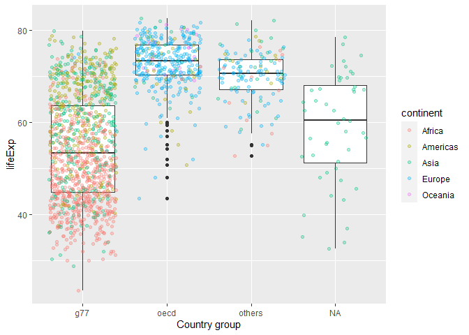
Compare lifeExp for OECD, G77, and other countries
gapminder_extended %>%
  ggplot(aes(x=g77_and_oecd_countries,y=lifeExp))+
    geom_boxplot()+
    geom_jitter(aes(color=continent), alpha=0.3)+
    labs(x="Country group")
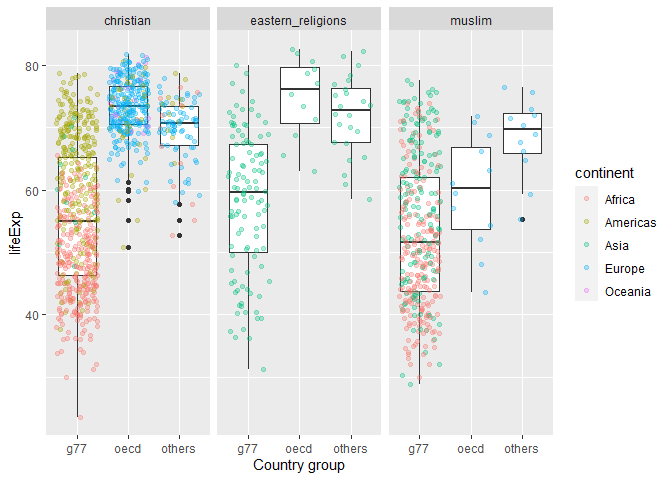
Compare lifeExp for OECD, G77, and other countries by most common religion
gapminder_extended %>%
  filter(main_religion_2008 %in% c("christian","eastern_religions","muslim")) %>%
  ggplot(aes(x=g77_and_oecd_countries,y=lifeExp))+
    geom_boxplot()+
    geom_jitter(aes(color=continent), alpha=0.3)+
    labs(x="Country group")+
    facet_wrap(~main_religion_2008)
Part 2
Gapminder data is only available from 1952 to 2007. What if we wanted to examine data after 2007 as well as population projections?
Download population size estimates by country from 1800 to 2100
population <- gsheet2tbl("https://docs.google.com/spreadsheets/d/14_suWY8fCPEXV0MH7ZQMZ-KndzMVsSsA5HdR-7WqAC0/edit#gid=176703676")
See what population data looks like
glimpse(population)
## Rows: 59,297
## Columns: 4
## $ geo        <chr> "afg", "afg", "afg", "afg", "afg", "afg", "afg", "afg", "af~
## $ name       <chr> "Afghanistan", "Afghanistan", "Afghanistan", "Afghanistan",~
## $ time       <dbl> 1800, 1801, 1802, 1803, 1804, 1805, 1806, 1807, 1808, 1809,~
## $ Population <dbl> 3280000, 3280000, 3280000, 3280000, 3280000, 3280000, 32800~
Only retain population estimates after 2007, rename variables to match gapminder variable names
population <- population %>%
  filter(time>2007) %>%
  rename(year=time, country=name, pop=Population) %>%
  select(-geo)
Add continent data to population from gapminder
# create a data frame listing continent for every country
continent <- gapminder %>%
  select(country, continent) %>%
  distinct()

# add continent data to population data frame
population <- left_join(population, continent, by = "country")

# see how many countries are missing continent data by continent
population %>%
  group_by(year) %>%
  summarise(missing_continent = sum(is.na(continent)))
## # A tibble: 93 x 2
##     year missing_continent
##    <dbl>             <int>
##  1  2008                61
##  2  2009                61
##  3  2010                61
##  4  2011                61
##  5  2012                61
##  6  2013                61
##  7  2014                61
##  8  2015                61
##  9  2016                61
## 10  2017                61
## # ... with 83 more rows
Use bind_rows() to stack population below gapminder
gapminder_pop <- bind_rows(gapminder, population) %>%
  arrange(country,year)
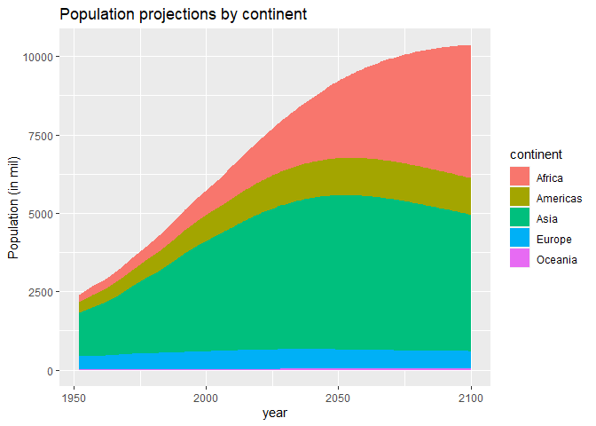
Visualize trends in population growth by continent
gapminder_pop %>%
  filter(!is.na(continent)) %>%
  group_by(continent, year) %>%
  summarise(pop=sum(pop)/1000000) %>%
  ggplot(aes(x=year, y=pop, fill=continent))+
  geom_area()+
  labs(title="Population projections by continent",
               y="Population (in mil)")
## `summarise()` has grouped output by 'continent'. You can override using the `.groups` argument.
Attributions
Written by Albina Gibadullina with input from Vincenzo Coia.